This post complements an earlier discussion of the Pareto distribution in a companion blog (found here). This post gives a side-by-side comparison of the Pareto type I distribution and Pareto type II Lomax distribution. We discuss the calculations of the mathematical properties shown in the comparison. Several of the properties in the comparison indicate that Pareto distributions (both Type I and Type II) are heavy tailed distributions. The properties presented in the comparison (and the thought processes behind them) are a good resource for studying actuarial exams.
The following table gives a side-by-side comparison for Pareto Type I and Pareto Type II.

![\displaystyle \begin{array}{llllllll} \text{ } &\text{.} & \text{ } & \text{ } & \text{ } & \text{ } & \text{ } &\text{ } \\ 8a &\text{Limited} &E[X \wedge d] & \text{ } & \text{ } & \text{ } & \displaystyle \frac{\theta}{\alpha-1} \biggl[1-\biggl(\frac{\theta}{d+\theta} \biggr)^{\alpha-1} \biggr] &\alpha \ne 1 \\ \text{ } & \text{Expectation} & \text{ } \\ \text{ } & \text{ } \\ 8b & \text{Limited} &E[X \wedge d] & \text{ } & \text{ } & \text{ } & \displaystyle -\theta \ \text{ln} \biggl(\frac{\theta}{d+\theta} \biggr) &\alpha = 1 \\ \text{ } & \text{Expectation} & \text{ } \\ \text{ } & \text{ } \\ 8c & \text{Limited} &E[(X \wedge d)^k] & \displaystyle \frac{\alpha \theta^k}{\alpha-k}-\frac{k \theta^\alpha}{(\alpha-k) d^{\alpha-k}} & \alpha>k & \text{ } & \text{See below} &\text{all } k \\ \text{ } & \text{Expectation} & \text{ } \\ \text{ } & \text{ } \\ 9 & \text{VaR} &VaR_p(X) & \displaystyle \frac{\theta}{(1-p)^{1/\alpha}} & \text{ } & \text{ } & \displaystyle \frac{\theta}{(1-p)^{1/\alpha}}-\theta &\text{ } \\ \text{ } & \text{ } \\ 10 &\text{TVaR} &TVaR_p(X) & \displaystyle \frac{\alpha}{\alpha-1} VaR_p(X) & \alpha>1 & \text{ } & \displaystyle \frac{\alpha}{\alpha-1} VaR_p(X)+\frac{\theta}{\alpha-1} &\alpha>1 \\ \text{ } & \text{ } \\ \end{array}](https://s0.wp.com/latex.php?latex=%5Cdisplaystyle+%5Cbegin%7Barray%7D%7Bllllllll%7D+%5Ctext%7B+%7D+%26%5Ctext%7B.%7D+%26+%5Ctext%7B+%7D+%26+%5Ctext%7B+%7D++%26+%5Ctext%7B+%7D++%26+%5Ctext%7B+%7D+%26+%5Ctext%7B+%7D++%26%5Ctext%7B+%7D+%5C%5C+8a+%26%5Ctext%7BLimited%7D+%26E%5BX+%5Cwedge+d%5D+%26+%5Ctext%7B+%7D++%26+%5Ctext%7B+%7D++%26+%5Ctext%7B+%7D+%26+%5Cdisplaystyle+%5Cfrac%7B%5Ctheta%7D%7B%5Calpha-1%7D+%5Cbiggl%5B1-%5Cbiggl%28%5Cfrac%7B%5Ctheta%7D%7Bd%2B%5Ctheta%7D+%5Cbiggr%29%5E%7B%5Calpha-1%7D+%5Cbiggr%5D++%26%5Calpha+%5Cne+1+%5C%5C++%5Ctext%7B+%7D+%26+%5Ctext%7BExpectation%7D+%26+%5Ctext%7B+%7D+%5C%5C++%5Ctext%7B+%7D+%26+%5Ctext%7B+%7D+%5C%5C++++++8b+%26+%5Ctext%7BLimited%7D+%26E%5BX+%5Cwedge+d%5D+%26+%5Ctext%7B+%7D++%26+%5Ctext%7B+%7D++%26+%5Ctext%7B+%7D+%26+%5Cdisplaystyle+-%5Ctheta+%5C+%5Ctext%7Bln%7D+%5Cbiggl%28%5Cfrac%7B%5Ctheta%7D%7Bd%2B%5Ctheta%7D+%5Cbiggr%29++%26%5Calpha+%3D+1+%5C%5C++++++++++%5Ctext%7B+%7D+%26+%5Ctext%7BExpectation%7D+%26+%5Ctext%7B+%7D+%5C%5C++%5Ctext%7B+%7D+%26+%5Ctext%7B+%7D+%5C%5C++++++8c+%26+%5Ctext%7BLimited%7D+%26E%5B%28X+%5Cwedge+d%29%5Ek%5D+%26+%5Cdisplaystyle+%5Cfrac%7B%5Calpha+%5Ctheta%5Ek%7D%7B%5Calpha-k%7D-%5Cfrac%7Bk+%5Ctheta%5E%5Calpha%7D%7B%28%5Calpha-k%29+d%5E%7B%5Calpha-k%7D%7D++%26+%5Calpha%3Ek++%26+%5Ctext%7B+%7D+%26+%5Ctext%7BSee+below%7D++%26%5Ctext%7Ball+%7D+k+%5C%5C+++++++%5Ctext%7B+%7D+%26++++%5Ctext%7BExpectation%7D+%26+%5Ctext%7B+%7D+%5C%5C++++%5Ctext%7B+%7D+%26+%5Ctext%7B+%7D+%5C%5C++++9+%26+%5Ctext%7BVaR%7D+%26VaR_p%28X%29+%26+%5Cdisplaystyle+%5Cfrac%7B%5Ctheta%7D%7B%281-p%29%5E%7B1%2F%5Calpha%7D%7D++%26+%5Ctext%7B+%7D++%26+%5Ctext%7B+%7D+%26+%5Cdisplaystyle+%5Cfrac%7B%5Ctheta%7D%7B%281-p%29%5E%7B1%2F%5Calpha%7D%7D-%5Ctheta++%26%5Ctext%7B+%7D+%5C%5C+++++++++++%5Ctext%7B+%7D+%26+%5Ctext%7B+%7D+%5C%5C++++10+%26%5Ctext%7BTVaR%7D+%26TVaR_p%28X%29+%26+%5Cdisplaystyle+%5Cfrac%7B%5Calpha%7D%7B%5Calpha-1%7D+VaR_p%28X%29++%26+%5Calpha%3E1++%26+%5Ctext%7B+%7D+%26+%5Cdisplaystyle+%5Cfrac%7B%5Calpha%7D%7B%5Calpha-1%7D+VaR_p%28X%29%2B%5Cfrac%7B%5Ctheta%7D%7B%5Calpha-1%7D+++%26%5Calpha%3E1+%5C%5C+++++++++++%5Ctext%7B+%7D+%26+%5Ctext%7B+%7D+%5C%5C++++%5Cend%7Barray%7D&bg=ffffff&fg=333333&s=0&c=20201002)
One item that is not indicated in the table is ![E[(X \wedge d)^k]](https://s0.wp.com/latex.php?latex=E%5B%28X+%5Cwedge+d%29%5Ek%5D&bg=ffffff&fg=333333&s=0&c=20201002) for Pareto Type II, which is given below.
for Pareto Type II, which is given below.
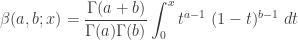
where  is the incomplete beta function, which is defined as follows:
for any  ,
,  and
and  .
.
Discussion
The above table describes two distributions that are called Pareto (Type I and Type II Lomax). Each of them has two parameters –  (shape parameter) and
  (scale parameter). The support of Pareto Type I is the interval
  . In other words, Pareto type I distribution can only take on real numbers greater than the scale parameter . On the other hand, the support of Pareto Type II is the interval
  . So a Pareto Type II distribution can take on any positive real numbers.
The two distributions are mathematically related. Judging from the PDF, it is clear that the PDF of Pareto Type II is the result of shifting Type I PDF to the left by the magnitude of (the same can be said about the CDF and survival function). More specifically, let  be a random variable that follows a Pareto Type I distribution with parameters and . Let
  . It is straightforward to verify that
  has a Pareto Type II distribution, i.e. its CDF and other distributional quantities are the same as the ones shown in the above table under Pareto Type II. If having the same parameters, the two distributions are essentially the same, in that each one is the result of shifting the other one by the amount .
A further indication that the two types are of the same distributional shape is that the variances are identical. Note that shifting a distribution to the left (or right) by a constant does not change the variance.
Since the two Pareto Types are the same distribution (except for the shifting), they share similar mathematical properties. For example, both distributions are heavy tailed distributions. In other words, they significantly put more probabilities on larger values. This point is discussed in more details below.
Calculation
First, the calculations. The moments are determined by the integral  where
where  is the PDF of the distribution in question. Because of the PDF for Pareto Type I is easy to work with, almost all the items under Pareto Type I are quite accessible. For example, the item 8c for Pareto Type I is calculated by the following integral.
In the remaining discussion, the focus is on Pareto Type II calculations.
The Pareto  th moment
  is definition the integral
  where is the Pareto Type II PDF. However, it is difficult to perform this integral. The best way to evaluate the moments in row 5 in the above table is to use the fact that Pareto Type II distribution is a mixture of exponential distributions with gamma mixing weight (see Example 2 here). Thus the moments of Pareto Type II can be obtained by integrating the conditional conditional th moment of the exponential distribution with gamma weight. The following shows the calculation.
In the above derivation, the conditional  is assumed to have an exponential distribution with mean
  . The random variable in turns has a gamma distribution with shape parameter and rate parameter . The integrand in the integral in the second to the last step is a gamma density, making the value of the integral 1.0. When is an integer, can be simplified as indicated in row 5.
The next calculation is the mean excess loss. It is the conditional expected value 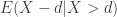 . If
. If  is an insurance loss and
  is some kind of threshold (e.g. the deductible in an insurance policy that covers this loss), then is the expected loss in excess of the threshold given that the loss exceeds . If is the lifetime of an individual, then is the expected remaining lifetime given that the individual has survived to age .
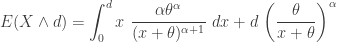
The expected value can be calculated by the integral  . This integral is not easy to evaluate when is a Pareto Type II PDF. Fortunately, there is another way to handle this calculation. The key idea is that if has a Pareto Type II distribution with parameters and (as described in the table), the conditional random variable
  also has a Pareto Type II distribution, this time with parameters and
  . The mean of a Pareto Type II distribution is always the ratio of the scale parameter to the shape parameter less one. Thus the mean of is as indicated in row 7 of the table.
The limited loss  is defined as follows.
One interpretation is that it is the insurance payment when the insurance policy has an upper cap on benefit. If the loss is below the cap , the insurance policy pays the loss in full. If the loss exceeds the cap , the policy only pays for the loss up to the limit . The expected insurance payment  is said to be the limited expectation. For Pareto Type II, the first moment can be evaluated by the following integral.
Integrating using a change of variable  will yield the results in row 8a and row 8b in the table, i.e. the cases for
  and
and  . A more interesting result is 8c, which is the th moment of the variable . The integral for this expectation can expressed using the incomplete beta function. The following evaluates the .
Further transform the integral in the above calculation by the change of variable using  .
.
The integrand in the last integral is the probability density function of the beta distribution with parameters  and
and  . Thus is as indicated in 8c.
Now we consider two risk measures – value-at-risk (VaR) and tail-value-at-risk (TVaR). The value-at-risk at security level  for a random variable is, denoted by
  , the
, the  th percentile of . Thus VaR is a fancy name for percentiles. Setting the Pareto Type II CDF equals to gives the VaR indicated in row 9 of the table. In other words, solving the following equation for
  gives the th percentile for Pareto Type II.
The tail-value-at-risk of a random variable at the security level , denoted by  , is the expected value of given that it exceeds . Thus
 ![TVaR_p(X)=E[X \lvert X>VaR_p(X)]](https://s0.wp.com/latex.php?latex=TVaR_p%28X%29%3DE%5BX+%5Clvert+X%3EVaR_p%28X%29%5D&bg=ffffff&fg=333333&s=0&c=20201002) . Letting
. Letting 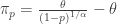 , the following integral gives the tail-value-at-risk for Pareto Type II. The integral is evaluated by the change of variable .
Tail Weight
Several properties in the above table show that the Pareto distribution (both types) is a heavy-tailed distribution. When a distribution significantly puts more probabilities on larger values, the distribution is said to be a heavy tailed distribution (or said to have a larger tail weight). There are four ways to look for indication that a distribution is heavy tailed.
- Existence of moments.
- Hazard rate function.
- Mean excess loss function.
- Speed of decay of the survival function to zero.
Tail weight is a relative concept – distribution A has a heavier tail than distribution B. The first three points are ways to tell heavy tails without a reference distribution. Point number 4 is comparative.
Existence of moments
For a given random variable  , the existence of all moments
  , for all positive integers , indicates a light (right) tail for the distribution of . The existence of positive moments exists only up to a certain value of a positive integer is an indication that the distribution has a heavy right tail.
Note that the existence of the Pareto higher moments is capped by the shape parameter (both Type I and Type II). Thus if  , only exists for
  . In particular, the Pareto Type II mean
  does not exist for
  . If the Pareto distribution is to model a random loss, and if the mean is infinite (when ), the risk is uninsurable! On the other hand, when
  , the Pareto variance does not exist. This shows that for a heavy tailed distribution, the variance may not be a good measure of risk.
As compared with Pareto, the exponential distribution, the Gamma distribution, the Weibull distribution, and the lognormal distribution are considered to have light tails since all moments exist.
Hazard rate function
The hazard rate function  of a random variable is defined as the ratio of the density function and the survival function.
The hazard rate is called the force of mortality in a life contingency context and can be interpreted as the rate that a person aged will die in the next instant. The hazard rate is called the failure rate in reliability theory and can be interpreted as the rate that a machine will fail at the next instant given that it has been functioning for units of time. It follows that the hazard rate of Pareto Type I is  and is
  for Type II. They are both decreasing function of .
Another indication of heavy tail weight is that the distribution has a decreasing hazard rate function. Thus the Pareto distribution (both types) is considered to be a heavy distribution based on its decreasing hazard rate function.
One key characteristic of hazard rate function is that it can generate the survival function.
Thus if the hazard rate function is decreasing in , then the survival function will decay more slowly to zero. To see this, let 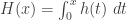 , which is called the cumulative hazard rate function. As indicated above, the survival function can be generated by
  . If is decreasing in ,
  is smaller than where is constant in or increasing in . Consequently is decaying to zero much more slowly than . Thus a decreasing hazard rate leads to a slower speed of decay to zero for the survival function (a point discussed below).
In contrast, the exponential distribution has a constant hazard rate function, making it a medium tailed distribution. As explained above, any distribution having an increasing hazard rate function is a light tailed distribution.
The mean excess loss function
Suppose that a property owner is exposed to a random loss . The property owner buys an insurance policy with a deductible such that the insurer will pay a claim in the amount of  if a loss occurs with
  . The insuerer will pay nothing if the loss is below the deductible. Whenever a loss is above , what is the average claim the insurer will have to pay? This is one way to look at mean excess loss function, which represents the expected excess loss over a threshold conditional on the event that the threshold has been exceeded. Thus the mean excess loss function is
  , a function of the deductible .
According to row 7 in the above table, the mean excess loss for Pareto Type I is  and for Type II is
 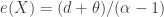 . They are both increasing functions of the deductible ! This means that the larger the deductible, the larger the expected claim if such a large loss occurs! If a random loss is modeled by such a distribution, it is a catastrophic risk situation.
In general, an increasing mean excess loss function is an indication of a heavy tailed distribution. On the other hand, a decreasing mean excess loss function indicates a light tailed distribution. The exponential distribution has a constant mean excess loss function and is considered a medium tailed distribution.
Speed of decay of the survival function to zero
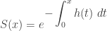
The survival function 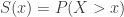 captures the probability of the tail of a distribution. If a distribution whose survival function decays slowly to zero (equivalently the cdf goes slowly to one), it is another indication that the distribution is heavy tailed. This point is touched on when discussing hazard rate function.
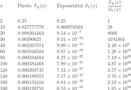
The following is a comparison of a Pareto Type II survival function and an exponential survival function. The Pareto survival function has parameters ( and
and  ). The two survival functions are set to have the same 75th percentile, which is
  . The following table is a comparison of the two survival functions.
Note that at the large values, the Pareto right tails retain much more probabilities. This is also confirmed by the ratio of the two survival functions, with the ratio approaching infinity. If a random loss is a heavy tailed phenomenon that is described by the above Pareto survival function ( and ), then the above exponential survival function is woefully inadequate as a model for this phenomenon even though it may be a good model for describing the loss up to the 75th percentile. It is the large right tail that is problematic (and catastrophic)!
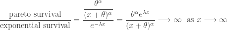
Since the Pareto survival function and the exponential survival function have closed forms, We can also look at their ratio.
In the above ratio, the numerator has an exponential function with a positive quantity in the exponent, while the denominator has a polynomial in . This ratio goes to infinity as  .
.
In general, whenever the ratio of two survival functions diverges to infinity, it is an indication that the distribution in the numerator of the ratio has a heavier tail. When the ratio goes to infinity, the survival function in the numerator is said to decay slowly to zero as compared to the denominator.
The Pareto distribution has many economic applications. Since it is a heavy tailed distribution, it is a good candidate for modeling income above a theoretical value and the distribution of insurance claims above a threshold value.

 2017 – Dan Ma

![\displaystyle E[(X \wedge d)^k]=\frac{\theta^k \Gamma(k+1) \Gamma(\alpha-k)}{\Gamma(\alpha)} \beta[k+1, \alpha-k; \frac{d}{d+\theta}]+d^k \biggl(\frac{\theta}{d+\theta} \biggr)^\alpha](https://s0.wp.com/latex.php?latex=%5Cdisplaystyle+E%5B%28X+%5Cwedge+d%29%5Ek%5D%3D%5Cfrac%7B%5Ctheta%5Ek+%5CGamma%28k%2B1%29+%5CGamma%28%5Calpha-k%29%7D%7B%5CGamma%28%5Calpha%29%7D+%5Cbeta%5Bk%2B1%2C+%5Calpha-k%3B+%5Cfrac%7Bd%7D%7Bd%2B%5Ctheta%7D%5D%2Bd%5Ek+%5Cbiggl%28%5Cfrac%7B%5Ctheta%7D%7Bd%2B%5Ctheta%7D+%5Cbiggr%29%5E%5Calpha&bg=ffffff&fg=333333&s=0&c=20201002)
![\displaystyle E[(X \wedge d)^k]=\int_\theta^d x^k \ \frac{\alpha \theta^\alpha}{x^{\alpha+1}} \ dx+d^k \ \biggl(\frac{\theta}{x}\biggr)^\alpha](https://s0.wp.com/latex.php?latex=%5Cdisplaystyle+E%5B%28X+%5Cwedge+d%29%5Ek%5D%3D%5Cint_%5Ctheta%5Ed+x%5Ek+%5C+%5Cfrac%7B%5Calpha+%5Ctheta%5E%5Calpha%7D%7Bx%5E%7B%5Calpha%2B1%7D%7D+%5C+dx%2Bd%5Ek+%5C+%5Cbiggl%28%5Cfrac%7B%5Ctheta%7D%7Bx%7D%5Cbiggr%29%5E%5Calpha&bg=ffffff&fg=333333&s=0&c=20201002)


![\displaystyle E[(X \wedge d)^k]=\int_0^d x^k \ \frac{\alpha \theta^\alpha}{(x+\theta)^{\alpha+1}} \ dx +d^k \ \biggl(\frac{\theta}{x+\theta}\biggr)^\alpha](https://s0.wp.com/latex.php?latex=%5Cdisplaystyle+E%5B%28X+%5Cwedge+d%29%5Ek%5D%3D%5Cint_0%5Ed+x%5Ek+%5C+%5Cfrac%7B%5Calpha+%5Ctheta%5E%5Calpha%7D%7B%28x%2B%5Ctheta%29%5E%7B%5Calpha%2B1%7D%7D+%5C+dx+%2Bd%5Ek+%5C+%5Cbiggl%28%5Cfrac%7B%5Ctheta%7D%7Bx%2B%5Ctheta%7D%5Cbiggr%29%5E%5Calpha&bg=ffffff&fg=333333&s=0&c=20201002)


![\displaystyle E[X \lvert X>VaR_p(X)]=\int_{\pi_p}^\infty x \ \frac{\alpha \theta^\alpha}{(x+\theta)^{\alpha+1}} \ x \ dx=\frac{\alpha}{\alpha-1} VaR_p(X)+\frac{\theta}{\alpha-1}](https://s0.wp.com/latex.php?latex=%5Cdisplaystyle+E%5BX+%5Clvert+X%3EVaR_p%28X%29%5D%3D%5Cint_%7B%5Cpi_p%7D%5E%5Cinfty+x+%5C+%5Cfrac%7B%5Calpha+%5Ctheta%5E%5Calpha%7D%7B%28x%2B%5Ctheta%29%5E%7B%5Calpha%2B1%7D%7D+%5C+x+%5C+dx%3D%5Cfrac%7B%5Calpha%7D%7B%5Calpha-1%7D+VaR_p%28X%29%2B%5Cfrac%7B%5Ctheta%7D%7B%5Calpha-1%7D&bg=ffffff&fg=333333&s=0&c=20201002)


Pingback: Practice Problem Set 4 – Pareto Distribution « Practice Problems in Actuarial Modeling
Pingback: More on Pareto distribution | Applied Probability and Statistics
Pingback: The Pareto distribution | Applied Probability and Statistics
Pingback: Practice Problem Set 5 – Exercises for Severity Models « Practice Problems in Actuarial Modeling
Pingback: Practice Problem Set 1 – method of moments estimation | SOA Exam C / CAS Exam 4
Pingback: More on calculating maximum likelihood estimators | SOA STAM Exam
Pingback: Practice Problem Set 13 – variance of insurance payment per loss | Practice Problems in Actuarial Modeling