Several versions of negative binomial distribution

This post shows how to work with negative binomial distribution from an actuarial modeling perspective. The negative binomial distribution is introduced as a Poisson-gamma mixture. Then other versions of the negative binomial distribution follow. Specific attention is paid to the thought processes that facilitate calculation involving negative binomial distribution.

Negative Binomial Distribution as a Poisson-Gamma Mixture

Here’s the setting for the Poisson-gamma mixture. Suppose that $X \lvert \Lambda$ has a Poisson distribution with mean $\Lambda$ and that $\Lambda$ is a random variable that varies according to a gamma distribution with parameters $\alpha$ (shape parameter) and $\rho$ (rate parameter). Then the following is the unconditional probability function of $X$ .

$\displaystyle (1) \ \ \ \ P[X=k]=\frac{\Gamma(\alpha+k)}{k! \ \Gamma(\alpha)} \ \biggl( \frac{\rho}{1+\rho} \biggr)^\alpha \ \biggl(\frac{1}{1+\rho} \biggr)^k \ \ \ \ k=0,1,2,3,\cdots$

The distribution described in (1) is one parametrization of the negative binomial distribution (derived here). It has two parameters $\alpha$ and $\rho$ (coming from the gamma mixing weights). The following is another parametrization.

$\displaystyle (2) \ \ \ \ P[X=k]=\frac{\Gamma(\alpha+k)}{k! \ \Gamma(\alpha)} \ \biggl( \frac{1}{1+\theta} \biggr)^\alpha \ \biggl(\frac{\theta}{1+\theta} \biggr)^k \ \ \ \ k=0,1,2,3,\cdots$

The distribution described in (2) is obtained when the gamma mixing weight $\Lambda$ has a shape parameter $\alpha$ and a scale parameter $\theta$ . Since the gamma scale parameter and rate parameter is related by $\rho=1/ \theta$ , (2) can be derived from (1) by setting $\rho=1/ \theta$ .

Both (1) and (2) contain the ratio $\frac{\Gamma(\alpha+k)}{k! \ \Gamma(\alpha)}$ that is expressed using the gamma function. The next task is to simplify the ratio using a general notion of binomial coefficient.

The Poisson-gamma mixture is discussed in this blog post in a companion blog called Topics in Actuarial Modeling.

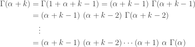
General Binomial Coefficient

The familiar binomial coefficient is the following:

$(3) \ \ \ \ \displaystyle \binom{n}{j}=\frac{n!}{j! (n-j)!}$

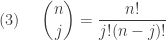
where the top number $n$ is a positive integer and the bottom number $j$ is a non-negative integer such that $n \ge j$ . Other notations for binomial coefficient are $C(n,j)$ , $_nC_j$ and $C_{n,j}$ . The right hand side of the above expression can be simplified by canceling out $(n-j)!$ .

$(4) \ \ \ \ \displaystyle \binom{n}{j}=\frac{n (n-1) (n-2) \cdots (n-(j-1))}{j!}$

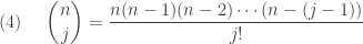
The expression in (4) is obtained by canceling out $(n-j)!$ in (3). Note that $n$ does not have to be an integer for the calculation in (4) to work. The bottom number $j$ has to be a non-negative number since $j!$ is involved. However, $n$ can be any positive real number as long as $n>j-1$ .

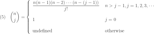
Thus the expression in (4) gives a new meaning to the binomial coefficient where $n$ is a positive real number and $j$ is a non-negative integer such that $n>j-1$ .

$\displaystyle (5) \ \ \ \ \binom{n}{j}=\left\{ \begin{array}{ll} \displaystyle \frac{n (n-1) (n-2) \cdots (n-(j-1))}{j!} &\ n>j-1, j=1,2,3,\cdots \\ \text{ } & \text{ } \\ \displaystyle 1 &\ j=0 \\ \text{ } & \text{ } \\ \displaystyle \text{undefined} &\ \text{otherwise} \end{array} \right.$

For example, $\binom{2.3}{1}=2.3$ and $\binom{5.1}{3}=(5.1 \times 4.1 \times 3.1) / 3!=10.8035$ . The thought process is that the numerator is obtained by subtracting 1 $j-1$ times from $n$ . If $j=0$ , this thought process would not work. For convenience, $\binom{n}{0}=1$ when $n$ is a positive real number.

We now use the binomial coefficient defined in (5) to simplify the ratio $\frac{\Gamma(\alpha+k)}{k! \ \Gamma(\alpha)}$ where $\alpha$ is a positive real number and $k$ is a non-negative integer. We use a key fact about gamma function: $\Gamma(1+w)=w \Gamma(w)$ . Then for any integer $k \ge 1$ , we have the following derivation.

$\displaystyle \begin{aligned} \Gamma(\alpha+k)&=\Gamma(1+\alpha+k-1)=(\alpha+k-1) \ \Gamma(\alpha+k-1) \\&=(\alpha+k-1) \ (\alpha+k-2) \ \Gamma(\alpha+k-2) \\&\ \ \ \vdots \\&=(\alpha+k-1) \ (\alpha+k-2) \cdots (\alpha+1) \ \alpha \ \Gamma(\alpha) \end{aligned}$

$\displaystyle \frac{\Gamma(\alpha+k)}{k! \ \Gamma(\alpha)}=\frac{(\alpha+k-1) \ (\alpha+k-2) \cdots (\alpha+1) \ \alpha}{k!}$

The right hand side of the above expression is precisely the binomial coefficient $\binom{\alpha+k-1}{k}$ when $k \ge 1$ . Thus we have the following relation.

$\displaystyle (6) \ \ \ \ \frac{\Gamma(\alpha+k)}{k! \ \Gamma(\alpha)}=\frac{(\alpha+k-1) \ (\alpha+k-2) \cdots (\alpha+1) \ \alpha}{k!}=\binom{\alpha+k-1}{k}$

where $k$ is an integer with $k \ge 1$ .

Negative Binomial Distribution

With relation (6), the two versions of Poisson-gamma mixture stated in (1) and (2) are restated as follows:

$\displaystyle (7) \ \ \ \ P[X=k]=\binom{\alpha+k-1}{k} \ \biggl( \frac{\rho}{1+\rho} \biggr)^\alpha \ \biggl(\frac{1}{1+\rho} \biggr)^k \ \ \ \ k=0,1,2,3,\cdots$

$\displaystyle (8) \ \ \ \ P[X=k]=\binom{\alpha+k-1}{k} \ \biggl( \frac{1}{1+\theta} \biggr)^\alpha \ \biggl(\frac{\theta}{1+\theta} \biggr)^k \ \ \ \ k=0,1,2,3,\cdots$

The above two parametrizations of negative binomial distribution are used if information about the Poisson-gamma mixture is known. In (7), the gamma distribution in the Poisson-gamma mixture has shape parameter $\alpha$ and rate parameter $\rho$ . In (8), the gamma distribution has shape parameter $\alpha$ and scale parameter $\theta$ . The following is a standalone version of the binomial distribution.

$\displaystyle (9) \ \ \ \ P[X=k]=\binom{\alpha+k-1}{k} \ p^\alpha \ (1-p)^k \ \ \ \ \ \ \ \ \ \ \ \ \ \ \ \ \ k=0,1,2,3,\cdots$

In (9), the negative binomial distribution has two parameters $\alpha>0$ and $p$ where $0<p<1$ . In this parmetrization, the parameter $p$ is simply a real number between 0 and 1. It can be viewed as a probability. In fact, this is the case when the parameter $\alpha$ is an integer. Version (9) can be restated as follows when $\alpha$ is an integer.

$\displaystyle \begin{aligned} (10) \ \ \ \ P[X=k]&=\binom{\alpha+k-1}{k} \ p^\alpha \ (1-p)^k \\&=\frac{(\alpha+k-1)!}{k! \ (\alpha-1)!} \ p^\alpha \ (1-p)^k \ \ \ \ \ \ \ \ \ \ \ \ \ \ \ \ \ k=0,1,2,3,\cdots \end{aligned}$

In version (10), the parameters are $\alpha$ (a positive integer) and a real number $p$ with $0<p<1$ . Since $\alpha$ is an integer, the usual binomial coefficient appears in the probability function.

Version (10) has a natural interpretation. A Bernoulli trial is an random experiment that results in two distinct outcome – success or failure. Suppose that the probability of success is $p$ in each trial. Perform a series of independent Bernoulli trials until exactly $\alpha$ successes occur where $\alpha$ is a fixed positive integer. Let the random variable $X$ be the number of failures before the occurrence of the $\alpha$ th success. Then (10) is the probability function for the random variable $X$ .

A special case of (10). When the parameter $\alpha$ is 1, the negative binomial distribution has a special name.

$\displaystyle (11) \ \ \ \ P[X=k]=p \ (1-p)^k \ \ \ \ \ \ \ \ \ \ \ \ \ \ \ \ \ \ \ \ \ \ \ \ \ \ \ \ \ \ \ \ \ \ k=0,1,2,3,\cdots$

The distribution in (11) is said to be a geometric distribution with parameter $p$ . The random variable $X$ defined by (11) can be interpreted as the number of failures before the occurrence of the first success when performing a series of independent Bernoulli trials. Another important property of the geometric distribution is that it is the only discrete distribution with the memoryless property. As a result, the survival function of the geometric distribution is $P[X>k]=(1-p)^{k+1}$ where $k=0,1,2,\cdots$ .

More about Negative Binomial Distribution

The probability functions of various versions of the negative binomial distribution have been developed in (1), (2), (7), (8), (9), (10) and (11). Other distributional quantities can be derived from the Poisson-gamma mixture. We derive the mean and variance of the negative binomial distribution.

Suppose that the negative binomial distribution is that of version (8). The conditional random variable $X \lvert \Lambda$ has a Poisson distribution with mean $\Lambda$ and the random variable $\Lambda$ has a gamma distribution with a shape parameter $\alpha$ and a scale parameter $\theta$ . Note that $E(\Lambda)=\alpha \theta$ and $Var(\Lambda)=\alpha \theta^2$ . Furthermore, we have the conditional mean and conditional variance

The following derives the mean and variance of $X$ .

$E(X)=E[E(X \lvert \Lambda)]=E[\Lambda]=\alpha \theta$

$\displaystyle \begin{aligned} Var(X)&=E[Var(X \lvert \Lambda)]+Var[E(X \lvert \Lambda)] \\&=E[\Lambda]+Var[\Lambda] \\&=\alpha \theta+\alpha \theta^2 \\&=\alpha \theta (1+\theta) \end{aligned}$

The above mean and variance are for parametrization in (8). To obtain the mean and variance for the other parametrizations, make the necessary translation. For example, to get (7), plug $\theta=\frac{1}{\rho}$ into the above mean and variance. For (9), let $p=\frac{1}{1+\theta}$ . Then solve for $\theta$ and plug that into the above mean and variance. Version (10) should have the same formulas as for (9). To get (11), set $\alpha=1$ . The following table lists the negative binomial mean and variance.

Version	Mean	Variance
(7)	$\displaystyle E(X)=\frac{\alpha}{\rho}$	$\displaystyle Var(X)=\frac{\alpha}{\rho} \ \biggl(1+\frac{1}{\rho} \biggr)$

(8)	$E(X)=\alpha \ \theta$	$Var(X)=\alpha \ \theta \ (1+\theta)$

(9) and (10)	$\displaystyle E(X)=\frac{\alpha (1-p)}{p}$	$\displaystyle Var(X)=\frac{\alpha (1-p)}{p^2}$

(11)	$\displaystyle E(X)=\frac{1-p}{p}$	$\displaystyle Var(X)=\frac{1-p}{p^2}$

The table shows that the variance of the negative binomial distribution is greater than its mean (regardless of the version). This stands in contrast with the Poisson distribution whose mean and the variance are equal. Thus the negative binomial distribution would be a suitable model in situations where the variability of the empirical data is greater than the sample mean.

Modeling Claim Count

The negative binomial distribution is a discrete probability distribution that takes on the non-negative integers $0,1,2,3,\cdots$ . Thus it can be used as a counting distribution, i.e. a model for the number of events of interest that occur at random. For example, the $X$ described above can be a good model for the frequency of loss, i,e, the random variable of the number of losses, either arising from a portfolio of insureds or from a particular insured in a given period of time.

The Poisson-gamma model has a great deal of flexibility. Consider a large population of individual insureds. The number of losses (or claims) in a year for each insured has a Poisson distribution with mean $\Lambda$ . From insured to insured, there is uncertainty in the mean annual claim frequency $\Lambda$ . However, the random variable $\Lambda$ varies according to a gamma distribution. As a result, the annual number of claims for an “average” insured or a randomly selected insured from the population will follow a negative binomial distribution.

Thus in a Poisson-gamma model, the claim frequency for an individual in the population follows a Poisson distribution with unknown gamma mean. The weighted average of these conditional Poisson claim frequencies is a negative binomial distribution. Thus the average claim frequency over all individuals has a negative binomial distribution.

The table in the preceding section shows that the variance of the negative binomial distribution is greater than the mean. This is in contrast to the fact that the variance and the mean of a Poisson distribution are equal. Thus the unconditional claim frequency $X$ is more dispersed than its conditional distributions. The increased variance of the negative binomial distribution reflects the uncertainty in the parameter of the Poisson mean across the population of insureds. The uncertainty in the parameter variable $\Lambda$ has the effect of increasing the unconditional variance of the mixture distribution of $X$ . Recall that the variance of a mixture distribution has two components, the weighted average of the conditional variances and the variance of the conditional means. The second component represents the additional variance introduced by the uncertainty in the parameter $\Lambda$ .

We present two examples. More examples to come at the end of the post.

Example 1
For a given insured driver in a large portfolio of insured drivers, the number of collision claims in a year has a Poisson distribution with mean $\Lambda$ . The Poisson mean $\Lambda$ follows a gamma distribution with mean 4 and variance 80. For a randomly selected insured driver from this portfolio,

what is the probability of having exactly 2 collision claims in the next year?
what is the probability of having at most one collision claim in the next year?

The number of collision claims in a year is a Poisson-gamma mixture and thus is a negative binomial distribution. From the given gamma mean and variance, we can determine the parameters of the gamma distribution. In this example, we use the parametrization of (8). Expressing the gamma mean and variance in terms of the shape and scale parameters, we have $\alpha \theta=4$ and $\alpha \theta^2=80$ . These two equations give $\alpha=0.2$ and $\theta=20$ . The probabilities are calculated based on (8).

$\displaystyle P[X=0]=\biggl( \frac{1}{21} \biggr)^{0.2}=0.5439$

$\displaystyle P[X=1]=\binom{0.2}{1} \ \biggl( \frac{1}{21} \biggr)^{0.2} \ \biggl( \frac{20}{21} \biggr)=0.2 \ \biggl( \frac{1}{21} \biggr)^{0.2} \ \biggl( \frac{20}{21} \biggr)=0.1036$

$\displaystyle P[X=2]=\binom{1.2}{2} \ \biggl( \frac{1}{21} \biggr)^{0.2} \ \biggl( \frac{20}{21} \biggr)^2=\frac{1.2 (0.2)}{2!} \ \biggl( \frac{1}{21} \biggr)^{0.2} \ \biggl( \frac{20}{21} \biggr)^2=0.0592$

The answer for the first question is $P[X=2]=0.0592$ . The answer for the second question is $P[X \le 1]=P[X=0]+P[X=1]=0.6475$ . Thus there is a closed to 65% chance that an insured driver has at most one claim in a year.

Example 2
For an automobile insurance company, the distribution of the annual number of claims for a policyholder chosen at random is modeled by a negative binomial distribution that is a Poisson-gamma mixture. The gamma distribution in the mixture has a shape parameters of $\alpha=1$ and scale parameter $\theta=3$ . What is the probability that a randomly selected policyholder has more than two claims in a year?

Since the gamma shape parameter is 1, the unconditional number of claims in a year is a geometric distribution with parameter $p=1/4$ . The following is the desired probability.

$\displaystyle P[X>2]=\biggl( \frac{1}{4} \biggr) \ \biggl( \frac{3}{4} \biggr)^3=\frac{27}{256}=0.1055$

A Recursive Formula

The probability functions described in (1), (2), (7), (8), (9), (10) and (11) describe clearly how the negative binomial probabilities are calculated based on the two given parameters. The probabilities can also be calculated recursively. Let $P_k=P[X=k]$ where $k=0,1,2,\cdots$ . We introduce a recursive formula that allows us to compute the value $P_k$ if $P_{k-1}$ is known. The following is the form of the recursive formula.

$\displaystyle (12) \ \ \ \ \frac{P_k}{P_{k-1}}=a+\frac{b}{k} \ \ \ \ \ \ \ \ \ \ k=1,2,3,\cdots$

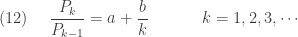
In (12), the numbers $a$ and $b$ are constants. Note that the formula (12) calculates probabilities $P_k$ for all $k \ge 1$ . It turns out that the initial probability $P_0$ is determined by the constants $a$ and $b$ . Thus the constants $a$ and $b$ completely determines the probability distribution represented by $P_k$ . Any discrete probability distribution that satisfies this recursive relation is said to be a member of the (a,b,0) class of distributions.

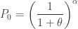
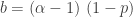
We show that the negative binomial distribution is a member of the (a,b,0) class of distributions. First, assume that the negative binomial distribution conforms to the parametrization in (8) with parameters $\alpha$ and $\theta$ . Then let $a$ and $b$ be defined as follows:

$\displaystyle a=\frac{\theta}{1+\theta}$

$\displaystyle b=\frac{(\alpha-1) \theta}{1+\theta}$ .

Let the initial probability be 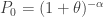$P_0=(1+\theta)^{-\alpha}$ . We claim that the probabilities generated by the formula (12) are identical to the ones calculated from (8). To see this, let’s calculate a few probabilities using the formula.

$\displaystyle P_0=\biggl(\frac{1}{1+\theta} \biggr)^\alpha$

$\displaystyle \begin{aligned} P_1&=(a+b) P_0 \\&=\biggl(\frac{\theta}{1+\theta}+ \frac{(\alpha-1) \theta}{1+\theta} \biggr) \ \biggl(\frac{1}{1+\theta} \biggr)^\alpha \\&=\alpha \ \biggl(\frac{1}{1+\theta} \biggr)^\alpha \ \frac{\theta}{1+\theta} \\&=\binom{\alpha}{1} \ \biggl(\frac{1}{1+\theta} \biggr)^\alpha \ \frac{\theta}{1+\theta}=P[X=1] \end{aligned}$

$\displaystyle \begin{aligned} P_2&=\biggl(a+\frac{b}{2} \biggr) P_1 \\&=\biggl(\frac{\theta}{1+\theta}+ \frac{(\alpha-1) \theta}{2(1+\theta)} \biggr) \ \alpha \ \biggl(\frac{1}{1+\theta} \biggr)^\alpha \ \frac{\theta}{1+\theta} \\&=\frac{(\alpha+1) \alpha}{2!} \ \biggl(\frac{1}{1+\theta} \biggr)^\alpha \ \biggl( \frac{\theta}{1+\theta} \biggr)^2 \\&=\binom{\alpha+1}{2} \ \biggl(\frac{1}{1+\theta} \biggr)^\alpha \ \biggl( \frac{\theta}{1+\theta} \biggr)^2=P[X=2] \end{aligned}$

$\displaystyle \begin{aligned} P_3&=\biggl(a+\frac{b}{3} \biggr) P_2 \\&=\biggl(\frac{\theta}{1+\theta}+ \frac{(\alpha-1) \theta}{3(1+\theta)} \biggr) \ \frac{(\alpha+1) \alpha}{2!} \ \biggl(\frac{1}{1+\theta} \biggr)^\alpha \ \biggl( \frac{\theta}{1+\theta} \biggr)^2 \\&=\frac{(\alpha+2) (\alpha+1) \alpha}{3!} \ \biggl(\frac{1}{1+\theta} \biggr)^\alpha \ \biggl( \frac{\theta}{1+\theta} \biggr)^3 \\&=\binom{\alpha+2}{3} \ \biggl(\frac{1}{1+\theta} \biggr)^\alpha \ \biggl( \frac{\theta}{1+\theta} \biggr)^3=P[X=3] \end{aligned}$

The above derivation demonstrates that formula (12) generates the same probabilities as (8). By adjusting the constants $a$ and $b$ , the recursive formula can also generate the probabilities in the other versions of the negative binomial distribution. For the negative binomial version (9) with parameters $\alpha$ and $p$ , the $a$ and $b$ should be defined as follows:

$a=1-p$

$b=(\alpha-1) \ (1-p)$

With the initial probability $P_0=p^\alpha$ , the recursive formula (12) will generate the same probabilities as those from version (9).

More Examples

Example 3
Suppose that an insured will produce $n$ claims during the next exposure period is

$\displaystyle \frac{e^{-\lambda} \ \lambda^n}{n!}$

where $n=0,1,2,3,\cdots$ . Furthermore, the parameter $\lambda$ varies according to a distribution with the following density function:

$\displaystyle g(\lambda)=\frac{9.261}{2} \ \lambda^2 \ e^{-2.1 \lambda} \ \ \ \ \ \ \lambda>0$

What is the probability that a randomly selected insured will produce more than 2 claims during the next exposure period?

Note that the claim frequency for an individual insured has a Poisson distribution with mean $\lambda$ . The given density function for the parameter $\lambda$ is that of a gamma distribution with $\alpha=3$ and rate parameter $\rho=2.1$ . Thus the number of claims in an exposure period for a randomly selected (or “average” insured) will have a negative binomial distribution. In this case the parametrization (7) is the most useful one to use.

$\displaystyle \begin{aligned} P(X=k)&=\binom{k+2}{k} \ \biggl(\frac{2.1}{3.1} \biggr)^3 \ \biggl(\frac{1}{3.1} \biggr)^k \\&=\frac{(k+2) (k+1)}{2} \ \biggl(\frac{21}{31} \biggr)^3 \ \biggl(\frac{10}{31} \biggr)^k \ \ \ \ \ k=0,1,2,3,\cdots \end{aligned}$

The following calculation gives the relevant probabilities to answer the question.

$\displaystyle P(X=0)=\biggl(\frac{21}{31} \biggr)^3$

$\displaystyle P(X=1)=3 \ \biggl(\frac{21}{31} \biggr)^3 \ \biggl(\frac{10}{31} \biggr)$

$\displaystyle P(X=2)=6 \ \biggl(\frac{21}{31} \biggr)^3 \ \biggl(\frac{10}{31} \biggr)^2$

Summing the three probabilities gives $P(X \le 2)=0.805792355$ . Then $P(X>2)=0.1942$ . There is a 19.42% chance that a randomly selected insured will have more than 2 claims in an exposure period.

Example 4
The number of claims in a year for each insured in a large portfolio has a Poisson distribution with mean $\lambda$ . The parameter $\lambda$ follows a gamma distribution with mean 0.75 and variance 0.5625.

Determine the proportion of insureds that are expected to have less than 1 claim in a year.

Setting $\alpha \theta=0.75$ and $\alpha \theta^2=0.5625$ gives $\alpha=1$ and $\theta=0.75$ . Thus the parameter $\lambda$ follows a gamma distribution with shape parameter $\alpha=1$ and scale parameter $\theta=0.75$ . This is an exponential distribution with mean 0.75. The problems asks for the proportion of insured with $\lambda<1$ . Thus the answer is $1-e^{-1/0.75}=0.7364$ . Thus about 74% of the insured population are expected to have less than 1 claim in a year.

Example 5
Suppose that the number of claims in a year for an insured has a Poisson distribution with mean $\Lambda$ . The random variable $\Lambda$ follows a gamma distribution with shape parameter $\alpha=2.5$ and scale parameter $\theta=1.2$ .

One thousand insureds are randomly selected and are to be observed for a year. Determine the number of selected insureds expected to have exactly 3 claims by the end of the one-year observed period.

With this being a Poisson-gamma mixture, the number of claims in a year for a randomly selected insured has a negative binomial distribution. Using (8) and based on the gamma parameters given, the following is the probability function of negative binomial distribution.

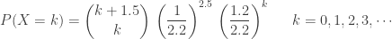
$\displaystyle P(X=k)=\binom{k+1.5}{k} \ \biggl(\frac{1}{2.2} \biggr)^{2.5} \ \biggl(\frac{1.2}{2.2} \biggr)^k \ \ \ \ \ k=0,1,2,3,\cdots$

The following gives the calculation for $P(X=3)$ .

$\displaystyle \begin{aligned} P(X=3)&=\binom{4.5}{3} \ \biggl(\frac{1}{2.2} \biggr)^{2.5} \ \biggl(\frac{1.2}{2.2} \biggr)^3 \\&=\frac{4.5 (3.5) (2.5)}{3!} \ \biggl(\frac{1}{2.2} \biggr)^{2.5} \ \biggl(\frac{1.2}{2.2} \biggr)^3 \\&=6.5625 \ \biggl(\frac{1}{2.2} \biggr)^{2.5} \ \biggl(\frac{1.2}{2.2} \biggr)^3 \\&=0.148350259 \end{aligned}$

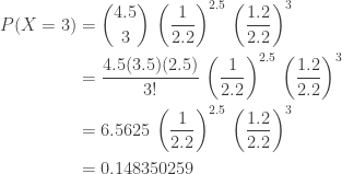
With $1000 \times 0.148350259=148.35$ , about 149 of the randomly selected insureds will have 3 claims in the observed period.

Example 6
Suppose that the annual claims frequency for an insured in a large portfolio of insureds has a distribution that is in the (a,b,0) class. Let $P_k$ be the probability that an insured has $k$ claims in a year.

Given that $P_1=0.3072$ , $P_2=0.12288$ and $P_3=0.04096$ , determine the probability that an insured has no claims in a one-year period.